
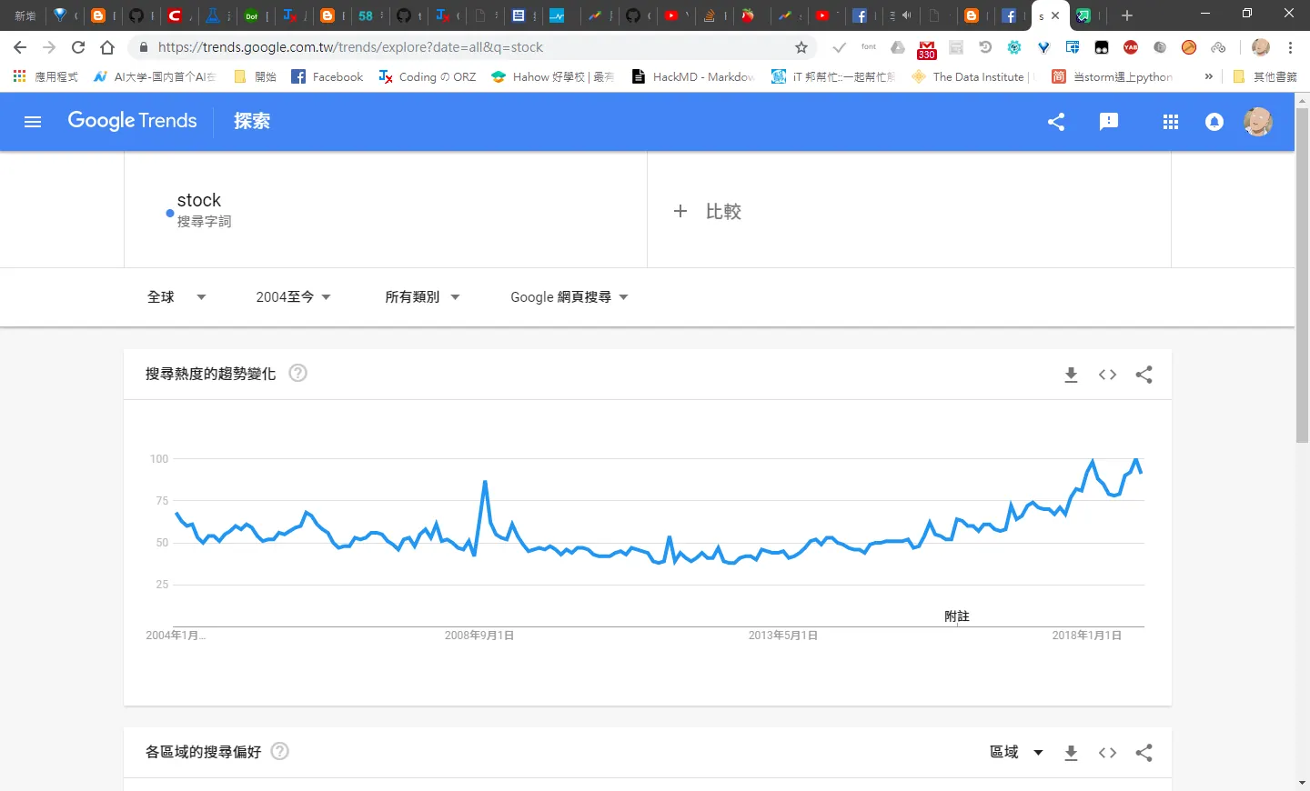
資料量可能會呈現全部趨向於100%的狀況
---
所以我打算先取得該年度區間所有的百分比再去*上每日百分比,這樣數據的呈現應該才是最準確的數字。
先取得2004至今的趨勢
程式碼
---
request.py
    def get_historical_interest2(self, keywords, year_start=2018, month_start=1, day_start=1, hour_start=0, year_end=2018, month_end=2, day_end=1, hour_end= 0, cat=0, geo='', gprop='', sleep=0):
        """Gets historical hourly data for interest by chunking requests to 1 week at a time (which is what Google allows)"""

        # construct datetime obejcts - raises ValueError if invalid parameters
        #start_date = datetime(year_start, month_start, day_start, hour_start)
        #end_date = datetime(year_end, month_end, day_end, hour_end)

        # the timeframe has to be in 1 week intervals or Google will reject it

        df = pd.DataFrame()

        tf = "all"
        try:
            self.build_payload(keywords,cat, tf, geo, gprop)
            week_df = self.interest_over_time()
            df = df.append(week_df)
            print (week_df)
        except Exception as e:
            print(e)
            pass

        return df
stockpytrend2.py
import numpy as np
import pandas as pd
import matplotlib.pyplot as plt
import scipy.stats as scs
from matplotlib import animation
from sklearn import preprocessing
from pytrends.request import TrendReq


# Login to Google. Only need to run this once, the rest of requests will use the same session.
pytrend = TrendReq()


tk = pytrend.get_historical_interest2(['stock'], year_start=2018, month_start=8, day_start=1, year_end=2018, month_end=8, day_end=1, cat=0, geo='', gprop='', sleep=0)

#tk.drop(['isPartial'], axis=1)
#del tk['isPartial']
print (tk.head())

plt.figure(figsize=(20,8))
fig, ax = plt.subplots()
#preprocessing.scale(tk['stock'])
ax.plot(tk['stock'])
plt.show()
運行結果
資料量問題
---
一開始我還以為要對資料做正規化,思考一下應該不是這問題,這邊會面臨到一直要數據被伺服器阻擋的問題(我先備份了數據)
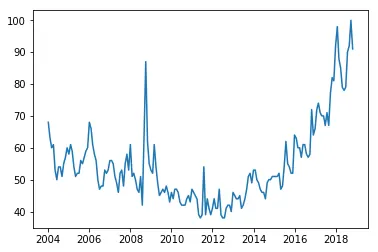 這是取得每月得數據
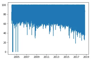 這是我們之前取得每日的數據
然後我們要對數據加工一下
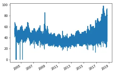 這才是正確的等比例數據
來看一下程式碼
這才是正確的等比例數據
來看一下程式碼
程式碼
---
import numpy as np
import pandas as pd
import csv
import matplotlib.pyplot as plt
import scipy.stats as scs
from matplotlib import animation
from sklearn import preprocessing
from pytrends.request import TrendReq
import datetime

date_time_str = '2018-06-29'
date_time_obj = datetime.datetime.strptime(date_time_str, '%Y-%m-%d')

df = pd.read_csv('googletrend_stock_data.csv', index_col='date', parse_dates=['date'])
price = df.squeeze()
price.head()


df = pd.read_csv('googletrend_stock_data2.csv', index_col='date', parse_dates=['date'])
all_price = df.squeeze()
all_price.head()
# print('Date:',date_time_str[5:7])
#Login to Google. Only need to run this once, the rest of requests will use the same session.
# pytrend = TrendReq()


# tk = pytrend.get_historical_interest2(['stock'], year_start=2004, month_start=1, day_start=1, year_end=2018, month_end=8, day_end=1, cat=0, geo='', gprop='', sleep=0)
# print(price)
# #tk.drop(['isPartial'], axis=1)
# #del tk['isPartial']
# print (tk.head())
# type(price)


def get_months( test):
    value = ""
    for i in range (0,len(all_price),1):
        if(test == str(all_price.index[i])[:7]+"-01 00:00:00"):
            value = all_price[str(all_price.index[i])[:7]+"-01 00:00:00"]
    return value

plt.figure(figsize=(16,8))
fig, ax = plt.subplots()

#preprocessing.scale(tk['stock'])
ax.plot(price)
plt.show()


# print( str(price.index[0])[:7] )
# print (price [price.index[0]])
s = pd.Series(price)

fuck = []
print (price.index)


for x in price.index:
    print (x)
    get_month = get_months(str(x)[:7]+"-01 00:00:00" )

    if(type(price[x]) == type(pd.Series(1))):
        fuck.append( [str(x),(np.float64(price[x][0])*(int(get_month)/100))])
    else:
        fuck.append( ([str(x),(np.float64(price[x])*(int(get_month)/100))]))

    #print (get_month/100)
    #print (price[x]*(get_month/100))

    #print (get_months(str(price.index[str(x)])[:7]+"-01 00:00:00"))

df2 = pd.DataFrame(fuck, columns = ['date', 'price'] )
df2['date'] = pd.to_datetime(df2['date'])
price2 = df2.set_index('date')


plt.figure(figsize=(16,8))

fig, ax = plt.subplots()

#preprocessing.scale(tk['stock'])
ax.plot(price2)
plt.gcf().autofmt_xdate()
plt.show()
Comments